DeepFake Detection Challenge

An overview of the process I went through for the DeepFake Detection Challenge hosted on Kaggle, where I achieved 15th position out of over 2000 teams (top 1%). This blog post is more a general guide of how I approached this competition than a technical report.

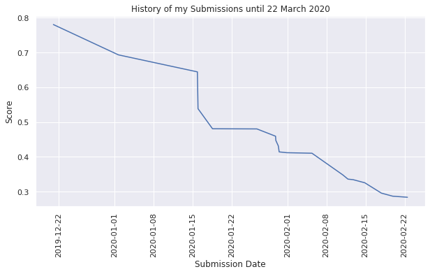
The competition ran from December 2019 to the end of March 2020 and was one of my first competitions in which I had enough resources to compete with top competitors as AWS sponsored participants with almost $2000 of AWS credits.

Competition Overview

The competition was set up such that generalisation in methods for identifying deep fakes was key to doing well in the competition. The scoring was divided into two leaderboards.

Public Leaderboard

The public leaderboard used a test set which was completely withheld and was similar to the training dataset. We could continuously run our models to check our score against competitors during the competition on this leaderboard.

Private Leaderboard

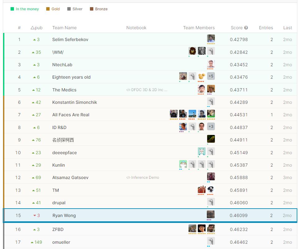
The private leaderboard had a different hidden test set which had videos similar to the training dataset as well as real, organic videos with and without deep fakes. The private leaderboard scores were only revealed at the end of the competition.

The competition metric used a log loss score, which would extremely punish predictions which were confident and wrong.

$$ LogLoss = -\frac{1}{n}\sum_{i=1}^{n} [y_i\log(\hat{y}_i)+(1-y_i)\log(1-\hat{y}_i)] $$

There was also a limit to using Kaggle kernels (notebooks) with a total external data size limit of 1GB and a 9 hour runtime limit for inference on around 1000 videos.

Data

The DFDC Dataset

The deep fake dataset for this challenge consists of over 500Gb of video data (around 200 000 videos). Each video contained around a 10 second clip of an actor or actors which were either the original ‘real’ video or a ‘fake’ video with altered facial or voice manipulations. The dataset was divided into 50 folders with under 500 actors in total. Majority of the videos contained facial manipulations compared to audio manipulation with around 8% of the dataset containing altered audio.

Data Preparations

I used videos from 4 randomly selected folders out of the 50 dataset folders as my validation dataset. The public unseen test set on Kaggle was around 50/50 split of real vs fake videos. I applied the same distribution to my validation set by choosing all the real videos and randomly selecting an equal number of fake videos from the 4 validation folders. This resulted in a validation set with just over 2000 videos. I also applied similar data augmentations, discussed in the forums, to the validation set where only one type of augmentation is applied per video. The distribution of my augmented validation dataset were as follows:

• 25% with frame level JPEG compression
• 25% with frame size reduced to 1/4 the original size
• 25% had the video frame rate reduced by half
• no augmentation to the remaining videos

Face Extraction

The input used for training was through selecting random frames of the full video resolution where each of the frames went through a pretrained face detector and extracting the cropped facial regions. These cropped facial regions are then resized to 224x224 and used as input into the deep fake detector network.

Augmentation

I used different input augmentations during training and updated the augmentation manually, depending on the CV score of the models. Initially the models were trained with only JPEG compression, downscaling, resizing and horizontal flipping. Upon further training more stronger versions of the above augmentation were applied along with other general pixel level augmentation such as adjustments to brightness, contrast and introducing noise. Full details of the coded implementation are available here.

Face Detector

The selected face detector was the pretrained MTCNN detector.

Margin Factor

Dynamic margins around the detected facial regions are used to include head features such as hair and ears of the facial crops. The margins are calculated based on the height of the facial region.

     margin = face_box_height/margin_factor - face_box_height

Where the margin_factor selected is 0.75.

Face Selection

The top 2 detected faces that have a probability above 0.99 are selected as input frames into the deep fake detector model. If no faces are found above the 0.99 threshold, then the next facial crop above the 0.6 threshold is used instead. If no faces are found by the face detector then the video is assumed to be 50% fake (to stop extreme punishment in the log loss score).

Models

As EfficientNet models produce state of the art results on various image classification tasks, many of my experiments used different versions of EfficientNet. For the frame by frame models I mainly used B6-EfficientNet model.

I did not want the sequence models to learn the same information as the frame by frame models so I avoided training the backbone of the network and trained only the head LSTM (2 hidden states) and fully connected layers of the network.

Initial experiments were on various ImageNet pretrained models (ResNet, EfficientNet, ResNeXt) as the backbone to the sequence classifier but these networks did not learn / learnt extremely slowly. My assumption for why these models were unable to learn is that the backbone component could not provide features to the LSTM which allowed it to distinguish between the real and fake faces. I switched the weights of my backbone network to one of the B6-EfficientNet models pre-trained on the frame by frame deep fake model which allowed the sequence model to learn much more quickly and had a slight improvement over using a frame by frame classifier.

Training

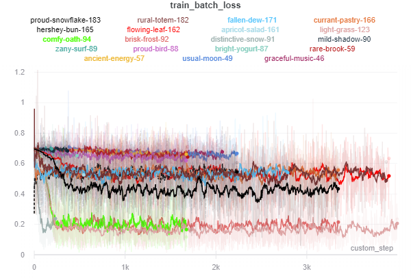
The training process involved managing the AWS credits effectively, with all my experiments on spot instances using the p3.2xlarge instances (single V100 GPU). I tracked my experiments with Weights and Biases, while starting and stopping experiments based on observations of the training and validation loss.

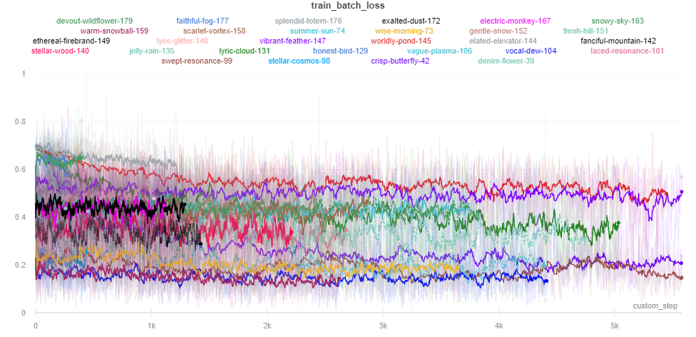
Overall, I had around 200 experiment for hyperparameter searching and model training. The training epochs took around 1.5 hours, which took a long time due to not doing intermediate preprocessing (something I would do in future competitions to save time and money).

List of ideas which I found helped speed up the training process and generalisation:

• CutMix augmentation (huge improvement in generalisation)
• Cyclic learning rate schedules
• AdamW optimiser
• Mixed precision using Nvidia Apex
• Half precision on the face detector model
• Stronger data augmentation as training progresses

Inference

I limited the number of frames analysed to 50 frames with 10 sequences per video to keep within the 9 hour inference limit. The frames were selected based on the following rules:

• Select 10 frames which are an equal distance apart
• Select 2 frames on either side of the selected frames to create the 5 frame sequence.

Post Processing

One of the key points of this competition was that if one frame contains a manipulated face then the output should predict “fake”. One method of using this knowledge in the model would be to choose the maximum prediction across all frames but this would be extremely risky due to the log loss scoring system. Similarly I found that using temperature scaling on predictions caused my CV to improve but the public leaderboard score decreased significantly. In order to enhance my predictions I used a post processing method based on the following rules:

• if the models predicted a certain number of frames to be over a threshold then select only those predictions which are over that threshold.
• Find the average of the predictions for that given threshold.
• Apply 2-3 times with different lower thresholds and a greater minimum number of selected frame values to be within the threshold.

These thresholds were found using a grid search across different minimum frame selections and threshold values for each model. I found this method to improve my score on the public leaderboard by between 0.02-0.04, with most improvements on the models trained with CutMix augmentation.

Audio

I set aside 2 weeks to look into audio classification. Having never worked with audio data before I tried many ideas but none of the models were able to learn at a level required to improve my score. The general process I used for the audio component involved converting the audio samples to a Mel Spectrogram which allowed audio task to be treated as an image classification task. The training process I followed was similar to one that achieved 1st Place on the public leaderboard for ERC2019. One of the issues with training models to find fake audio was the limited fake audio samples. Having limited success with the audio component I decided not to include these models in my final submission.

Ensemble

My final ensemble consisted of 3 models:

• An image classification models based on B6-EfficientNet trained without CutMix
• An image classification models based on B6-EfficientNet trained with CutMix
• A sequence classification model with a the B6-EfficientNet model as the backbone architecture and a head network with a 2 hidden state LSTM

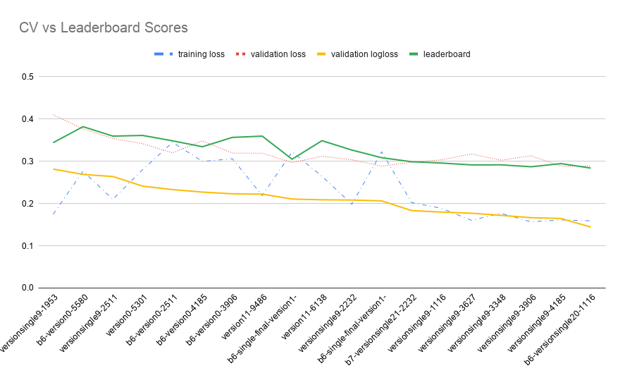
The selected models were ensembled by averaging the predictions together after the post processing.

Conclusions

Overall I am quite happy with my score and position on the leaderboard especially since I was able to remain in the top 20 teams for the public and private leaderboard. My initial goal was to reach 0.25 on the public leaderboard which I was able to achieve by getting 0.24397 (the lower the better). By participating in previous Kaggle competitions I was able to learn quite a lot from them and applied that knowledge to this competition. This competition also allowed me to perform many experiments thanks to the AWS Credits, which gave me more insights into hyperparameter tuning and optimising the model training process.